Tread

Diffusion models have become the cornerstone of visual generation, yet they continue to face challenges like sample inefficiency and high training costs. While traditional diffusion transformers struggle with quadratic complexity, much of the research has focused on reducing tokens through techniques like masking. In contrast, TREAD (2501.04765) takes a different approach by retaining token information via predefined routing pathways that strategically reintroduce data at deeper layers of the model. This method leverages multiple routing paths while incorporating an adaptive auxiliary loss, significantly boosting training efficiency without requiring architectural changes.

Quadratic Complexity

Starting off with the main problem the paper addresses - when a system has quadratic complexity relative to input length, it means the computational cost (time/memory) scales with the square of the input size. For example:

If the input length is \(N\), the cost grows as \(O(N^{2})\).
Doubling the input length \((2N)\) quadruples the computational cost \((4N^{2})\).

If the architecture scales quadratically with input length, training becomes prohibitively expensive for large inputs (e.g., high-resolution images, long videos). For instance:

A 256×256 image split into 16×16 patches becomes 256 tokens.
A transformer would compute \(256^2\) = 65,536 interactions per layer.

One way of reducing such tokens is masking but the paper introduces avoiding token discarding:
In many transformer architectures (especially for images/video), tokens (e.g., image patches) are discarded or merged early to reduce computational cost. For example:

Patch merging (e.g., in Vision Transformers): Combine neighboring patches into fewer tokens.
Token pruning: Remove "less important" tokens based on heuristics.

It risks losing fine-grained spatial or temporal information critical for tasks like image/video generation. Instead of discarding tokens, the authors store and reuse them via predefined pathways. Here’s how this works:

Token Preservation: Early-layer tokens (e.g., high-resolution details) are stored in memory.
Reintroduction to Deeper Layers: These tokens are later fused with processed features at deeper layers (e.g., via skip connections or cross-attention).
Efficiency Gains: By avoiding recomputation of discarded tokens, the model retains critical information without the full quadratic cost at every layer.

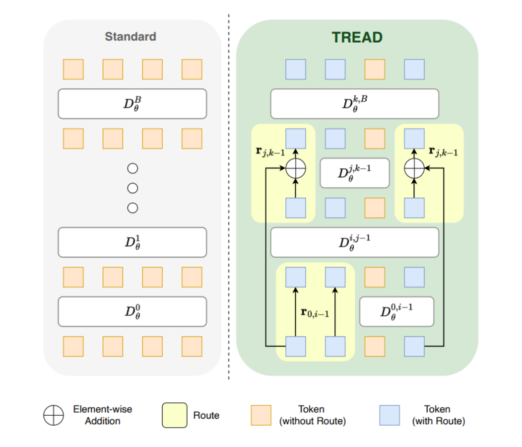
Analogy: Highway Networks for Tokens Think of predefined routes as "highways" that let tokens bypass intermediate layers. They’re stored in a memory buffer and merged back into the main network at specific depths, avoiding unnecessary processing. This is similar to: Skip connections in ResNets (but for tokens, not feature maps). Cross-attention in transformers (where stored tokens act as memory keys/values).

Routes: Token Highways for Efficient Computation

The paper introduces routes - Which essentially serves as a unidirectional transport for the tokens across layers. formal defination of a route \(r\) in the network architecture is designed to enable flexible information pathways through skip connections, enhancing training efficiency and preserving critical details:
A route \(r\) is formally defined as:

\( r = \{ (D_{li}^\theta, D_{lj}^\theta) \mid 0 \leq i \lt j \leq B \} \)

where \(B+1\) are the total layers in the network \(D^\theta\) indexed from 0 (input) to \(B\) (output).
Layer set: \( L = \{ D_{l1}^\theta, D_{l2}^\theta, \dots, D_{lB}^\theta \} \), representing the processing layers.
connection pairs: each pair denotes a direct pathway from layer \(l_{i}\) to layer \(l_{j}\), where \(i\) < \(j\).

The architecture emplyes smaller skips maybe to improve gradient flow during backprop and to mitigate vanishing gradients.

When the route \(r_{i,j}\) is active, the tokens are bypassed by all intermediate layers it spans. Once the route completes, these tokens become available again, allowing layer \( D_\theta^{l_{j}}\) to receive information from layer \( D_\theta^{l_{i}}\). An interesting point from the paper is they hypothesize that the semantic importance of the noise space plays a crucial role. By repeatedly supplying information about \(x_{t}\) to the network, the learning of the noise-image mapping becomes more efficient. hence the route \(r_{0,j}\) in the above figure.

With this each route \(r_{i,j}\) decreases the computational cost along its length, as tokens are not involved in any computation up to their reintroduction but also increases the memory footprint as you will have to store the tokens up till reintroduction.

Multiple Routes for further acceleration

Promoting exploration of multiple routes at once, ensuring that more segments of the network can access the noise-space information more regularly. But this is much more complex then using a single route ( Things are not always linear \(:(\) ). Now the complexity arrises as and when the first route \(r_{0,i}\) terminates, tokens are transferred from the input to layer \( D_\theta^{l_{i+1}}\), filling the set of tokens back up to its original size. With this an entirly new set of tokens are created, now the paper suggests on two objectives that should be considered while working with multiple routes :

Introducing \(x_{t}\) via route \(r_{j,k}\) to layer \( D_\theta^{l_{k+1}}\),
Utilizing the already computed information from the layers between \(r_{0,i}\) and \(r_{j,k}\) to utilize the models capacity efficiently.

To address these objectives the paper prefers using a linear combination of \(x_{t}\) and the representation produced by the direct predecessor of \(r_{j,k}\).

Leveraging Layer Similarities

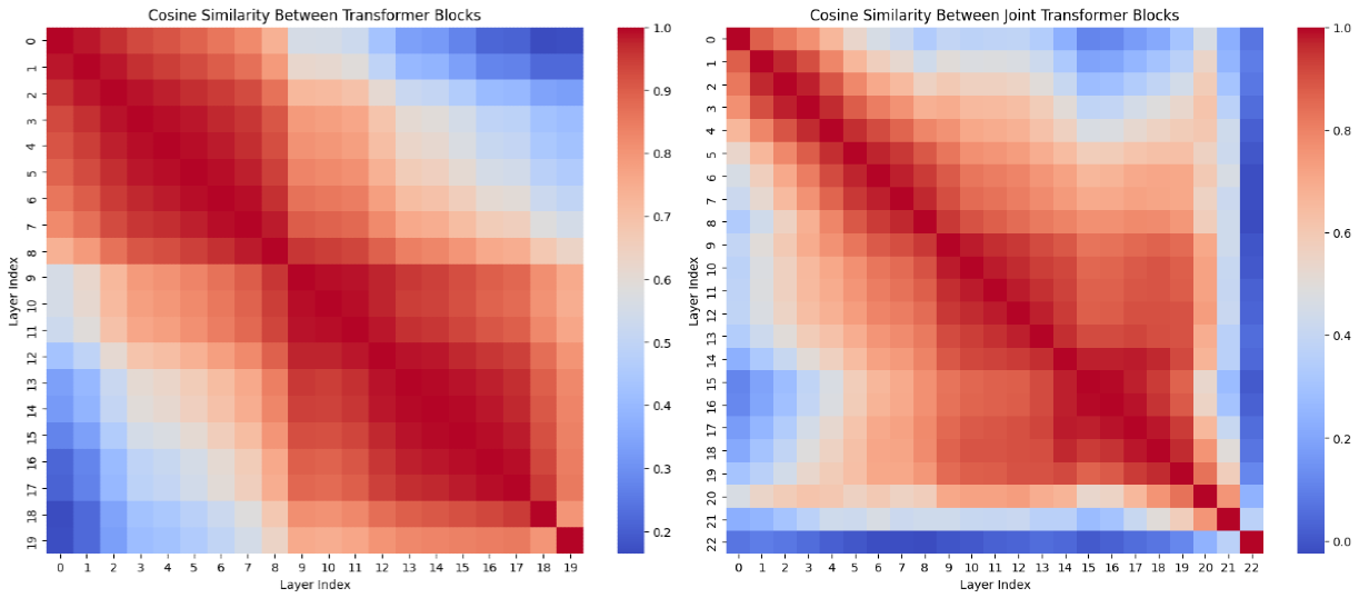
The above figure represents cosine similarities between Sana transformer blocks and SD3.5L Joint transformer blocks.

I think observed pattern of cosine similarities between layers presents an opportunity for optimizing route selection in multi-route architectures. When two layers exhibit high cosine similarity (e.g., > 0.8), their representations likely capture related features. This suggests that tokens passing through these layers might benefit from selective routing or skipping to avoid redundant transformations. layers with lower similarity scores might represent critical transformation points where full token processing is essential. \[ R(i, j) = \{ t \in T \mid s(i, j) > \tau \land f(t, i) \approx f(t, j) \} \]

\(T\) is the token set
\(f(t,l)\) is the feature representation of token \(t\) at layer \(l\)
\(R(i,j)\) defines the set of tokens that can safely utilize the route from layer \(i\) to \(j\)

If someone with the curious mind wants to dive into the details there is an amazing blog from Abhinay at HuggingFace Articles or here's a short tweet from me on the same topic on X/Twitter.

Multi-Route Ensemble Loss.

In the above sections we saw that withholding tokens increases task complexity. the added complexity can be managed by adjusting the loss functions, since traditional loss functions can only handle one mask at a time using multiple routes requirests handling multiple masks simultaneously. Each route \(r_{i,j}\) has it own mask operator \(m\), where \(V^k_{m}\) selects tokens for route based on random mask \(m\), \( \overline{V}^k_m \) is the complement operator (selects tokens NOT in the mask), there approch essentailly creates a more sophisticaed loss calculation system that can handle the complexity of having multiple information pathways. \[ L_{\text{dsm}}^k = \mathbb{E}_{x_0 \sim p_{\text{data}}, n \sim \mathcal{N}(0, t^2 I), m} \\ \| \overline{V}_m^k \left( D_\theta^{R^k} (x_0 + n, t) - x_0 \right) \|^2, \] \[ L_{\text{mae}}^k = \mathbb{E}_{x_0 \sim p_{\text{data}}, n \sim \mathcal{N}(0, t^2 I), m} \\ \| V_m^k \left( D_\theta^{R^k} (x_0 + n, t) - x_0 \right) \|^2 \] with this, where \(D_\theta^{R^k}(·,·)\) represents the subnetwork of \(D_\theta(·,·)\) defined by the k-th route in \(R\). Our final multi-route ensemble loss is formulated as \(L\): \[ L = \frac{1}{N} \sum_{k=1}^N L_{\text{dsm}}^k + \lambda L_{\text{mae}}^k \] where \(N\) denotes the total number of sequential routes employed.

Conclusion: The Magic of Routes

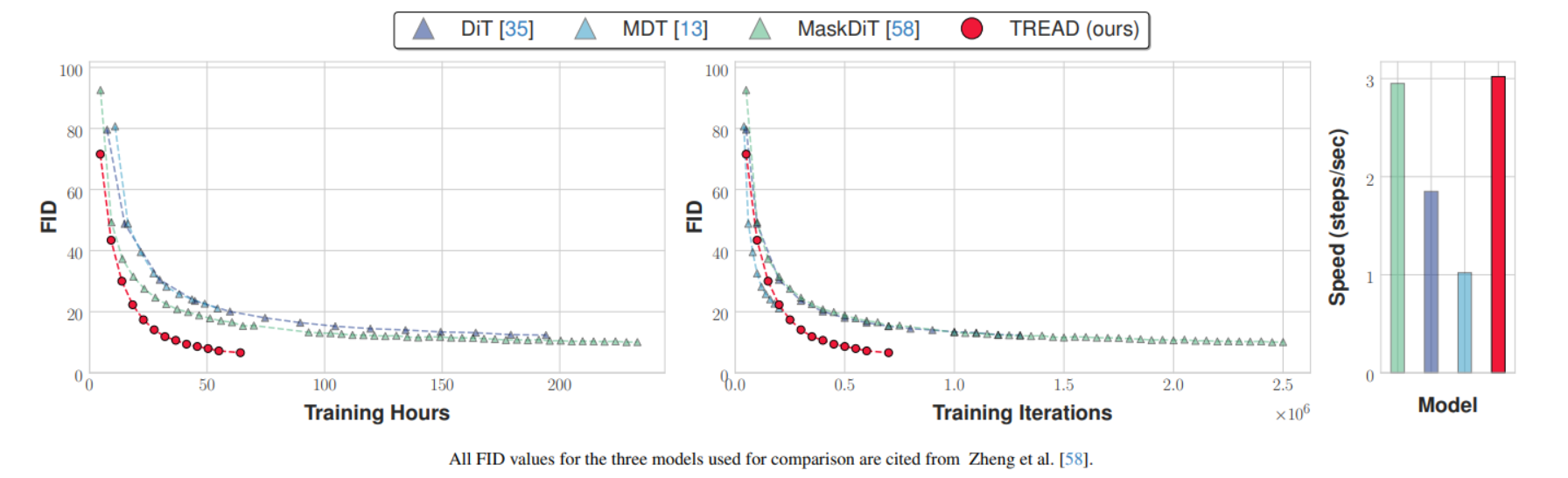
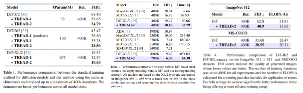
The paper mentions all the training strategies benchmarking on ImageNet-1K, which is a good PoC but they did not evaluate with the same setup, but hey it's legit lab though I feel there method has to be very sensitive to the hyperparameters, including masking rate and loss weighting, I would recomend going through there setup mentioned an the paper. Just mentioning the interesting things here starting off with FID score comparisons accross the paper. 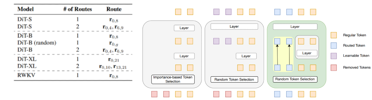I don't really like how they mention DiT all over the paper and the Implementation details are for training EDM ! anyways on that they ensure that the first route starts at \(D_\theta^{l_{0}}\) to maximize the potential length of route \(r\) spans. Now comparing pruning/ masking and routing, where both the approches would remove tokens in one way or the other routing forces you to use all the tokens merely witholding them from some computational blocks. All in all an interesting read though still requires a full scale test should be exiting experimenting with SANA ;), here's there codebase CompVis/tread.